Convolutional Neural Networks for Signals Processing: Implementation and challenges: Part1, Basic Convolutional layers
- ahatia0503
- November 4, 2024
- 12:36 pm
- No Comments

Convolutional Neural Networks therotical background
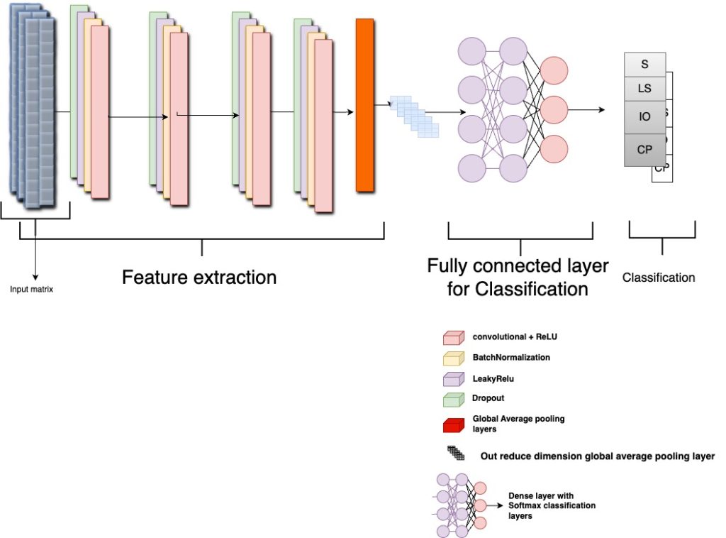
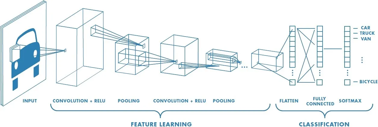
Convolutional Neural Networks (CNNs) are one of the most popular deep learning algorithms specialised in working signals, images, and videos and excelling most working on images and three-dimensional video. Different types of Convolutional Neural Networks, such as 1D Convolutional neural networks, can handle 1D data, such as signals and 1D matrices. The Deep learning algorithm is becoming quite very popular in signals processing as their 1D implementation that is very accurate for handling signals with very accurate performance compared to most well-known signal processing such as wavelet transform, Fourier transform, wavelet packet energy and different statistical methods such as moving average methods. 1D Convolutional neural network layers can be summarised as the following :
Convolutional layer
Relu layer and leaky Relu activation function
action function is used to introduce nonlinearit which is essential for learning a complet pattern in the data Relu is defined as: {ReLU}(x) = max(0, x)Leaky relu
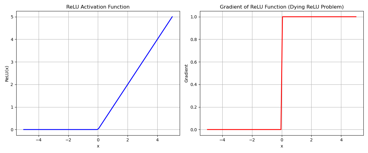
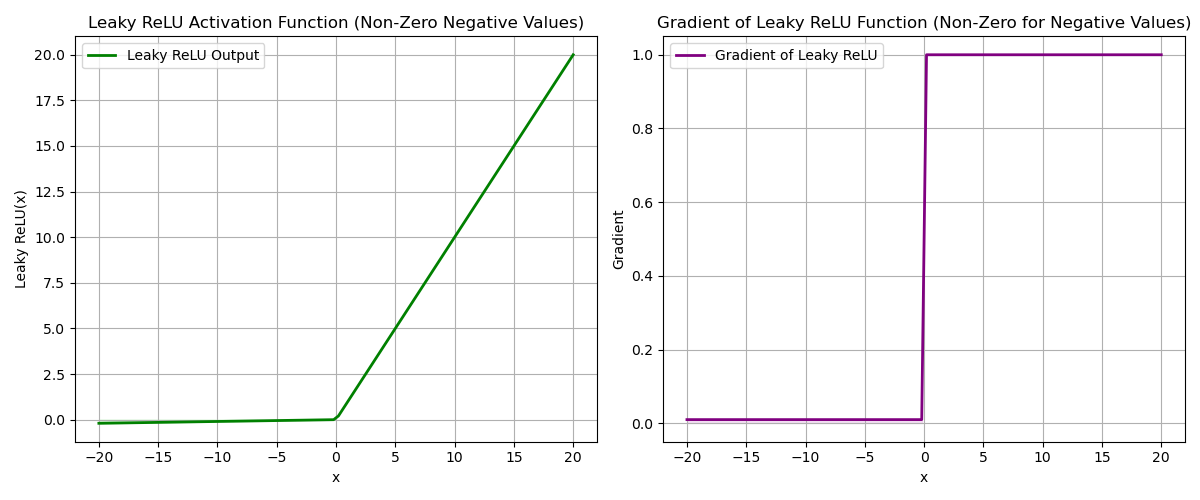
Leaky ReLU is used to solve the problem of dying ReLU, as it allows for a small gradient for negative inputs. See Figure 2 for more details.
 Figure 2: ReLU activation and gradient, illustrating the dying ReLU problem.
See Figure 3 for an illustration of Leaky ReLU.
 Figure 3: Leaky ReLU activation and gradient, solving the dying ReLU problem.
Batch Normalization
Batch normalization is a technique designed to address internal covariate shift by normalizing the input to each layer in a neural network. However, some studies suggest that the exact reasons behind the observed improvements remain unclear, emphasizing the need for further experimental investigation. While internal covariate shift is widely regarded as a primary factor in convergence difficulties within neural architectures, batch statistics appear to be the key component in mitigating this shift. In contrast, the affine transformation may play a less significant role in this process. (Ioffe.et all).
Batch Normalization Equations Batch Normalization Techniques Batch Normalization Techniques
1. Batch Normalization (BN)
Normalization:
\[ \hat{x}_i = \frac{x_i - \mu_B}{\sqrt{\sigma_B^2 + \epsilon}} \]
Affine Transformation:
\[ y_i = \gamma \hat{x}_i + \beta \]
- \( x_i \)
- Input activation.
- \( \mu_B \)
- Mean of the mini-batch.
- \( \sigma_B^2 \)
- Variance of the mini-batch.
- \( \epsilon \)
- Small constant for numerical stability.
- \( \gamma \)
- Learnable scale parameter.
- \( \beta \)
- Learnable shift parameter.
2. Layer Normalization (LN)
Normalization:
\[ \hat{x}_i = \frac{x_i - \mu_L}{\sqrt{\sigma_L^2 + \epsilon}} \]
Affine Transformation:
\[ y_i = \gamma \hat{x}_i + \beta \]
- Input activation: \( x_i \)
- \( \mu_L \)
- Mean of the layer's activations.
- Variance of the layer's activations: \( \sigma_L^2 \)
- \( \epsilon \)
- Small constant for numerical stability.
- \( \gamma \)
- Learnable scale parameter.
- \( \beta \)
- Learnable shift parameter.
One of the unique layers of the neural networks works by kernel multiplication over each bit in the input matrix. Each filter slide of the input matrix makes an input-wise multiplication. These different filters during the element-wise multiplication help the CNNs to learn different features like edges and texture. While in the case of the signals, CNNs learn from temporal and frequency patterns. Another important feature that is learnable during the training is hierarchical Feature Learning; CNNs learn to capture increasingly different features. In the initial layer, CNNs tend to learn fundamental patterns such as (amplitude peaks and low frequency frequency oscillation). The deep layers are specialised to learn deep features within the signals, such as patterns associated with specific features or anomalies.

Activation Functions in Python
Sigmoid Activation Function
The sigmoid function maps input values to a range between 0 and 1.
import numpy as np

def sigmoid(x):
    return 1 / (1 + np.exp(-x))
Usage: Commonly used in binary classification tasks.
Hyperbolic Tangent (Tanh) Activation Function
The tanh function maps input values to a range between -1 and 1.
import numpy as np

def tanh(x):
    return np.tanh(x)
Usage: Often used in hidden layers of neural networks.
Rectified Linear Unit (ReLU) Activation Function
ReLU outputs the input if it's positive; otherwise, it returns zero.
import numpy as np

def relu(x):
    return np.maximum(0, x)
Usage: Widely used in hidden layers due to its simplicity and effectiveness.
Leaky ReLU Activation Function
Leaky ReLU allows a small, non-zero gradient when the input is negative.
import numpy as np

def leaky_relu(x, alpha=0.01):
    return np.where(x > 0, x, alpha * x)
Usage: Helps mitigate the "dying ReLU" problem by allowing a small gradient for negative inputs.
Softmax Activation Function
Softmax converts a vector of values into a probability distribution.
import numpy as np

def softmax(x):
    e_x = np.exp(x - np.max(x))
    return e_x / e_x.sum(axis=0)
Usage: Typically used in the output layer for multi-class classification problems.
References
S. Ioffe and C. Szegedy. Batch Normalization: Accelerating Deep Network Training by Reducing Internal Covariate Shift. In Proceedings of the 32nd International Conference on Machine Learning (ICML), 2015.
A. L. Maas, A. Y. Hannun, and A. Y. Ng. Rectifier Nonlinearities Improve Neural Network Acoustic Models. In Proceedings of the 30th International Conference on Machine Learning (ICML), 2013.
Conclusion
In this article, we introduced the basic architecture of Convolutional Neural Networks (CNNs). These foundational layers form the core of CNNs, particularly for tasks such as image or signal classification. Typically, a fully connected layer follows the residual architecture in CNNs. CNNs serve as powerful automatic feature extractors in signal processing, although other tools, like wavelet transforms, wavelet packet energy, and complex mode indicator functions, can be used as handcrafted feature extractors for signals. In future articles, we will delve deeper into various CNN architectures and their applications in signal processing, exploring the learnable parameters and feature maps they produce at each layer. Through experimental investigations and coding examples, we aim to provide a comprehensive understanding of this critical scientific field, which lays the foundation for generative models and large language models.