Thinktechway

Feature Selection methods and advantages

Feature selection is a crucial step in the process of building machine learning models. By selecting the most relevant features, we can improve model performance, increase interpretability, and reduce computational cost. Feature selection methods help in identifying and eliminating irrelevant or redundant features, ensuring that the model remains efficient and effective. Feature selection, as a dimensionality reduction technique, aims to choosing a small subset of the relevant features from the original features by removing irrelevant, redundant or noisy features. Feature selection usually can lead to better learning performance, i.e., higher learning accuracy, lower computational cost, and better model interpretability. Recently, researchers from computer vision, text mining and so on have proposed a variety of feature selection algorithms and in terms of theory and experiment, show the effectiveness of their works.

Feature Selection Methods

Feature Selection Methods: Advantages and Disadvantages

<
Feature Selection Techniques

Feature Selection Techniques: Mathematical Background

1. Filter Methods

Filter methods evaluate each feature individually using statistical criteria like correlation, mutual information, and chi-square tests.

  • Pearson’s Correlation Coefficient: Measures the linear relationship between two continuous variables.

Formula:

$$ r = \frac{\sum (X_i - \bar{X})(Y_i - \bar{Y})}{\sqrt{\sum (X_i - \bar{X})^2 \sum (Y_i - \bar{Y})^2}} $$
  • Mutual Information: Measures the shared information between two variables.

Formula:

$$ I(X; Y) = \sum_{x \in X} \sum_{y \in Y} p(x, y) \log \frac{p(x, y)}{p(x) p(y)} $$
  • Chi-Square Test: Evaluates the association between categorical variables.

Formula:

$$ \chi^2 = \sum \frac{(O_i - E_i)^2}{E_i} $$

2. Wrapper Methods

Wrapper methods involve training models with subsets of features and evaluating their performance to identify the best combination.

  • Recursive Feature Elimination (RFE): RFE removes the least important features iteratively based on the model’s coefficients.

Linear Model Example:

$$ y = \beta_0 + \beta_1 x_1 + \beta_2 x_2 + \dots + \beta_n x_n $$

3. Embedded Methods

Embedded methods perform feature selection during model training.

  • Lasso Regression: Adds an \( L_1 \) penalty to the model to encourage sparsity, shrinking some coefficients to zero.

Cost Function:

$$ \min_{\beta} \left( \frac{1}{2n} \sum_{i=1}^{n} (y_i - X_i \beta)^2 + \lambda \sum_{j=1}^{p} |\beta_j| \right) $$

4. Dimensionality Reduction Techniques

These techniques transform the dataset into a lower-dimensional space while retaining the most information.

  • Principal Component Analysis (PCA): Finds the directions that capture the most variance in the data.

Formula:

$$ Z = X W $$

Where \( W \) contains the eigenvectors of the covariance matrix corresponding to the largest eigenvalues.


5. Heuristic and Evolutionary Methods

Heuristic methods, such as genetic algorithms, search for optimal feature subsets by mimicking evolutionary processes.

  • Genetic Algorithm: Uses operations like selection, crossover, and mutation to find the best feature combination.

Fitness Function:

$$ f(S) = \text{Model Accuracy with feature subset } S $$
Equation Example with KaTeX Minimal Stylish Article
“”

1. Information Gain (IG)

Information Gain measures the reduction in entropy when splitting a dataset based on a feature. It helps to select features by evaluating how much information a feature provides about the target variable.

The formula for Information Gain is:

$$ IG(Y, X) = H(Y) - H(Y | X) $$

Where \( H(Y) \) is the entropy of the target variable:

$$ H(Y) = -\sum_{i=1}^{n} p(y_i) \log_2 p(y_i) $$

\( H(Y | X) \) is the conditional entropy of the target variable given the feature.


2. Chi-Square Test (\(\chi^2\))

The Chi-Square Test determines the relationship between categorical features and the target. It compares observed and expected frequencies to determine if the feature significantly impacts the target variable.

The formula for the Chi-square statistic is:

$$ \chi^2 = \sum \frac{(O_i - E_i)^2}{E_i} $$

Where \( O_i \) is the observed frequency and \( E_i \) is the expected frequency.


3. Fisher’s Score

Fisher’s Score ranks features based on their ability to discriminate between different classes. Features with higher Fisher’s Scores are more useful for classification tasks.

The formula for Fisher’s Score is:

$$ F_j = \frac{(\mu_1 - \mu_2)^2}{\sigma_1^2 + \sigma_2^2} $$

Where \( \mu_1 \) and \( \mu_2 \) are the means of the feature values for the two classes, and \( \sigma_1^2 \) and \( \sigma_2^2 \) are the variances for the two classes.


4. Variance Threshold

The Variance Threshold method removes features with variance below a specified threshold. Features with low variance do not contribute much to distinguishing between samples.

The formula for the variance of a feature is:

$$ \text{Var}(X) = \frac{1}{n} \sum_{i=1}^{n} (x_i - \bar{x})^2 $$

Where \( x_i \) is the feature value for the \( i^{th} \) sample, and \( \bar{x} \) is the mean of the feature values.

Feature Correlation Visualizations Feature Selection Plots

Feature Selection Plots in Machine Learning

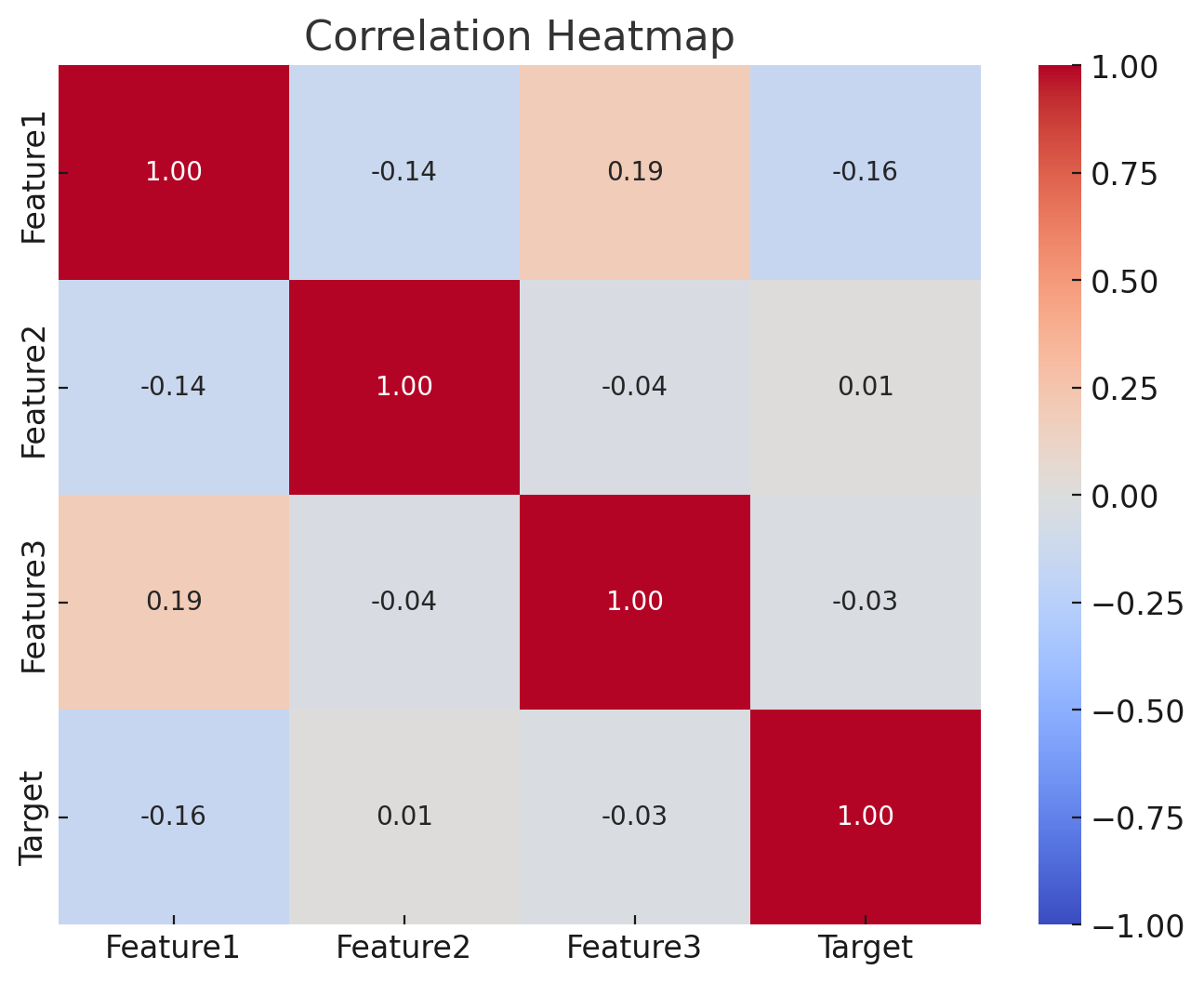
1. Correlation Heatmap

The heatmap visualizes the pairwise correlations between all features and the target. Highly correlated features can be dropped to avoid redundancy. There are many plots to identift the correlation between the feature correlation and deside on feature selection.

Correlation Heatmap

here is the code for Scatter plot Matrix

import seaborn as sns
import matplotlib.pyplot as plt

# Generate correlation heatmap
plt.figure(figsize=(8, 6))
sns.heatmap(data.corr(), annot=True, cmap='coolwarm', vmin=-1, vmax=1, fmt=".2f")
plt.title("Correlation Heatmap")
plt.show()
    

2. Scatter Plot Matrix (Pair Plot)

A scatter plot matrix visualizes relationships between pairs of features. This plot helps identify correlated features and outliers.

Scatter Plot Matrix
sns.pairplot(data, hue='Target')
plt.show()
    

3. Box Plot

A box plot compares the distribution of feature values across different target classes. Features with clear separations between classes are often good predictors.

Box Plot

here is the code for box plot

sns.boxplot(x='Target', y='Feature1', data=data)
plt.title("Box Plot of Feature1 vs Target")
plt.show()
    

4. Feature Importance Plot

This plot shows how important each feature is in a Random Forest model. Features with low importance can be dropped.

Feature Importance Plot

here is the code for feature important plot

from sklearn.ensemble import RandomForestClassifier

model = RandomForestClassifier()
X = data.drop('Target', axis=1)
y = data['Target']
model.fit(X, y)

importances = model.feature_importances_
plt.barh(X.columns, importances)
plt.title("Feature Importance Plot")
plt.show()
    

5. Variance Threshold Plot

This plot visualizes the variance of each feature. Features with very low variance do not contribute much to the model.

Variance Threshold Plot

here is the code for varience threehold plot

from sklearn.feature_selection import VarianceThreshold

selector = VarianceThreshold(threshold=0.1)
selector.fit(X)

variances = selector.variances_
plt.barh(X.columns, variances)
plt.title("Variance of Features")
plt.show()
    

6. PCA (Explained Variance Plot)

This plot shows how much variance each principal component explains. It helps decide how many components to keep in PCA.

PCA Explained Variance Plot
 

here is the code for varience threehold plot

from sklearn.decomposition import PCA pca = PCA().fit(X) explained_variance = pca.explained_variance_ratio_ plt.plot(range(1, len(explained_variance) + 1), explained_variance, marker='o') plt.title("Explained Variance by Principal Components") plt.xlabel("Number of Components") plt.ylabel("Explained Variance") plt.show()

Next article will delve deeper into feature selection

Facebook
Twitter
LinkedIn

Leave a Comment

Your email address will not be published. Required fields are marked *

Scroll to Top
Feature Selection Method Advantages Disadvantages
Filter Methods
  • Computational Efficiency: Faster and less resource-intensive
  • Model Agnosticity: Independent of specific machine learning algorithms
  • Suitable for high-dimensional data
  • Potential for Suboptimality: May not identify the best feature subset
  • Limited Consideration of Interactions: Overlooks complex relationships between features
Wrapper Methods
  • Higher Predictive Accuracy: Optimizes for the chosen model
  • Interaction Awareness: Considers feature interactions to maximize performance
  • Computational Complexity: Expensive and slow for large datasets
  • Risk of Overfitting: Prone to overfitting, especially with small datasets
Embedded Methods
  • Balance of Efficiency and Accuracy: Incorporated into model training for better results
  • Reduced Overfitting: Regularizes the feature selection process
  • Model Specificity: Often designed for specific algorithms
  • Potential for Complexity: Can still be computationally expensive for complex models